Documentation for pyLCSIM¶

Introduction¶

pyLCSIM is a python package to simulate X-ray lightcurves from coherent signals and power spectrum models.

Coherent signals can be specified as a sum of one or more sinusoids, each with its frequency, pulsed fraction and phase shift; or as a series of harmonics of a fundamental frequency (each with its pulsed fraction and phase shift).

Power spectra can be simulated from a model of the power spectrum density (PSD), using as a template one or more of the built-in library functions. The user can also define his/her custom models. Models are additive.

A PDF version of these notes is available here.

Warning: the current release (0.x.y) is HIGHLY EXPERIMENTAL! Use at your own risk...

Prerequisites¶

pyLCSIM requires Numpy (at least v1.8) and Astropy (at least v0.3).

Matplotlib is highly recommended if you want to plot your simulations.

Installation¶

The most straightforward way to install pyLCSIM is to use the Python Package Index and its pip utility (may require administrator privileges):

$ pip install pyLCSIM

To upgrade from a previous version:

$ pip install pyLCSIM --upgrade

The package source can be also downloaded here.

The installation in this case follows the usual steps:

$ tar xzvf pyLCSIM-0.x.y.tar.gz

$ cd pyLCSIM-0.x.y

$ python setup.py install

The last step may require administrator privileges.

Mailing list¶

A dedicated mailing list is available, to host announcements of new releases, to report issues and to get support. If interested, subscribe here.

License¶

The package is distributed under the MIT license.

Example 1¶

Let’s begin with a PSD model simulation.

We import the usual packages:

import matplotlib.pyplot as plt
import numpy as np
import pyLCSIM

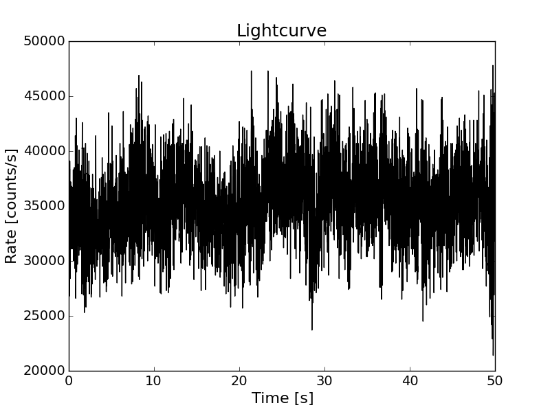
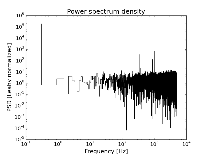
We assume that our source has a rate of 30000 counts/s. Moreover, we have a 5000 counts/s background rate, and we have made a 50 s exposure. Our observation has a time resolution of 10 ms. We want to simulate a QPO at a frequency of 10 Hz, superimposed to a continuum modelled as a smoothly-varying broken power law (spectral indices 1 and 2, with a steepness change at 1 Hz). The required fractional RMS variation of the signal is 1%:

rate_src    = 30000.0
rate_bkg    = 5000.0
t_exp       = 50.0
dt          = 0.01
frms        = 0.1

The total bins of the lightcurve are therefore:

nbins = t_exp/dt

The simulation follows as:

# Instantiate a simulation object
sim = pyLCSIM.Simulation()

# Add two PSD models: a smooth broken power law and a Lorentzian representing a QPO.
# See the documentation for details.
sim.addModel('smoothbknpo', [1., 1, 2, 1])
sim.addModel('lorentzian', [10., 1., 10, 2])

# Run the simulation
sim.run(dt, nbins, rate_src, rms=frms)

# Add Poisson noise to the light curve
sim.poissonRandomize(dt, rate_bkg)

# Get lightcurve and power spectrum as 1-D arrays
time, rate = sim.getLightCurve()
f, psd = sim.getPowerSpectrum()

Done! We can save the results as FITS files:

# Save FITS files with lightcurve and spectrum
pyLCSIM.saveFITSLC("myLC.fits", time, rate)
pyLCSIM.saveFITSPSD("myPSD.fits", f, psd)

and view the results:

# Plot the lightcurve and power spectrum
fig0 = plt.figure()
plt.plot(time, rate)
plt.xlabel("Time [s]")
plt.ylabel("Rate [counts/s]")
plt.title("Lightcurve")

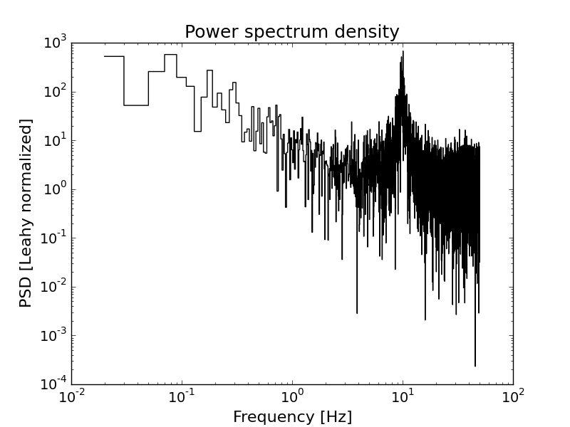
fig1 = plt.figure()
plt.loglog(f, psd, drawstyle='steps-mid', color='black')
plt.xlabel("Frequency [Hz]")
plt.ylabel("PSD [Leahy normalized]")
plt.title("Power spectrum density")

plt.show()

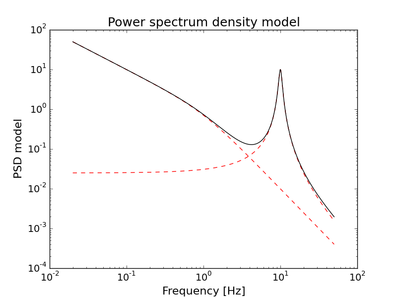
The PSD model used in the simulation can be obtained (and plotted) following the next example code:

freq_m, model_tot, model_comp = sim.getPSDModel(dt, nbins)
plt.figure()
for mod in model_comp:
        # Plot the various additive component as dashed lines
        plt.loglog(freq_m, mod, ls='dashed', color='red')
# Plot the total model
plt.loglog(freq_m, model_tot)
plt.show()

Example 2¶

The user can also define his/her own PSD models, simply as python functions. The only caveat is that the function should be positive-valued, and it is suggested to avoid too small output values.

The following example shows a simulation using an user-defined function (a Gaussian centered at 10 Hz, in this case):

def myFunc(f, p):
    """
    Example of user-defined function: a Gaussian.
    User-defined PSD models should be positive-valued!
    Moreover, in this example the output is clipped at 1e-32 to avoid too small values.
    """
    f = p[0]*np.exp(-(f-p[1])**2/p[2]**2)
    return np.clip(f, 1e-32, np.max(f))

sim = pyLCSIM.Simulation()
sim.addModel('smoothbknpo', [1., 1, 2, 1])
sim.addModel(myFunc, [1000., 10, 1.])

# Run the simulation
sim.run(dt, nbins, rate_src, rms=frms)

Additionally, PSD models can be also defined as astropy.modeling.models functions.

The following example is equivalent to the previous one (a Gaussian centered at 10 Hz):

from astropy.modeling import models

sim = pyLCSIM.Simulation()
sim.addModel('smoothbknpo', [1., 1, 2, 1])
# For astropy.modeling.models, you should define a dictionary of parameters instead of the usual list:
sim.addModel(models.Gaussian1D, {'amplitude':1000., 'mean':10., 'stddev':1.})

# Run the simulation
sim.run(dt, nbins, rate_src, rms=frms)

Example 3¶

The following example shows the simulation of a coherent signal using a sum of sinusoids:

import matplotlib.pyplot as plt
import numpy as np
import pyLCSIM

rate_src    = 30000.0
rate_bkg    = 5000.0
t_exp       = 1.0
dt          = 0.0001
nbins = t_exp/dt

Note the different exposure time (1 s) and time resolution (100 us):

# Instantiate a simulation object, this time as coherent
sim = pyLCSIM.Simulation(kind='coherent')

# Run the simulation, using:
# four sinusoidal frequencies: 340, 550, 883, 1032 Hz;
# with pulsed fractions 10%, 5%, 7% and 15% respectively;
# the third frequency has a 35 degree phase shift with respect to the others
sim.run(dt, nbins, rate_src, freq=[340, 550, 883, 1032], amp=[0.1, 0.05, 0.07, 0.15], phi=[0., 0, 35., 0.])

# Add Poisson noise to the light curve
sim.poissonRandomize(dt, rate_bkg)

# Get lightcurve and power spectrum as 1-D arrays
time, rate = sim.getLightCurve()
f, psd = sim.getPowerSpectrum()

# Plot the lightcurve and power spectrum
fig0 = plt.figure()
plt.plot(time, rate)
plt.xlabel("Time [s]")
plt.ylabel("Rate [counts/s]")
plt.title("Lightcurve")

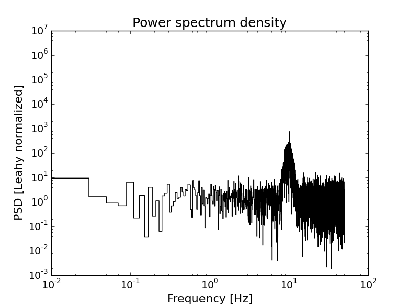
fig1 = plt.figure()
plt.loglog(f, psd, drawstyle='steps-mid', color='black')
plt.xlabel("Frequency [Hz]")
plt.ylabel("PSD [Leahy normalized]")
plt.title("Power spectrum density")

# Save FITS files with lightcurve and spectrum
pyLCSIM.saveFITSLC("myLC.fits", time, rate)
pyLCSIM.saveFITSPSD("myPSD.fits", f, psd)

plt.show()

Example 4¶

Finally, an example with a fundamental frequency and two harmonics:

import matplotlib.pyplot as plt
import numpy as np
import pyLCSIM

rate_src    = 300000.0
rate_bkg    = 3000.0
t_exp       = 1.0
dt          = 0.0001
phase_shift = 0.
nbins = t_exp/dt

# Instantiate a simulation object, this time as coherent
sim = pyLCSIM.Simulation(kind='coherent')


# Run the simulation:
# Fundamental at 500 Hz, 3 harmonics (500, 1000, 1500 Hz)
# with pulsed fractions 10%, 5% and 15% respectively
sim.run(dt, nbins, rate_src, freq=500, nha=3, amp=[0.1, 0.05, 0.15])

# Add Poisson noise to the light curve
sim.poissonRandomize(dt, rate_bkg)

# Get lightcurve and power spectrum as 1-D arrays
time, rate = sim.getLightCurve()
f, psd = sim.getPowerSpectrum()

# Plot the lightcurve and power spectrum
fig0 = plt.figure()
plt.plot(time, rate)

fig1 = plt.figure()
plt.loglog(f, psd, drawstyle='steps-mid', color='black')

# Save FITS files with lightcurve and spectrum
pyLCSIM.saveFITSLC("myLC.fits", time, rate)
pyLCSIM.saveFITSPSD("myPSD.fits", f, psd)

plt.show()

Main module¶

class pyLCSIM.Simulation(kind='psd')¶

Main simulation class.

History:

v1.3: Added getPSDModel method. Riccardo Campana, 2014.

v1.2: Added reset method. Riccardo Campana, 2014.

v1.1: Bugfix. Riccardo Campana, 2014.

v1: Initial python implementation. Riccardo Campana, 2014.

addModel(modelName, modelParams)¶: Append simulation model to model dictionary

getLightCurve()¶: Get lightcurve as time and rate arrays

getPSDModel(dt, nbins, freq=1000)¶: Get PSD model Returns a tuple with: frequency array, total model, array with single components

getPowerSpectrum()¶: Get power spectrum as frequency and power arrays

info()¶: Prints simulation informations

poissonRandomize(dt, bkg)¶: Add Poissonian noise to lightcurve (and background, if present)

reset()¶: Reset the simulation, emptying models array and other members

run(dt, nbins_old, mean, rms=None, freq=None, nha=None, amp=None, phi=None, verbose=False)¶: Run the simulation

pyLCSIM.lcsinusoid(dt=1.0, nbins=65536, mean=0.0, freq=None, nha=1, amp=None, phi=None, verbose=False)¶

Generate coherent signals as a sequence of sinusoids (if len(freq) > 1) or of the fundamental frequency plus nha-1 harmonics (if len(freq) == 1), each with normalized pulsed fraction amp[i].

Kwargs:

dt: time resolution of the lightcurve to be simulated (default: 1.0).

nbins: Number of bins of the simulated lightcurve (default: 65536).

freq: if float: frequency of the fundamental harmonic, if array: frequencies of sinusoids.

nha: number of harmonics (>1)

amp: array with nha/nfreq elements; pulsed fraction for each frequency

phi: array with nha/nfreq elements; phases (in degrees!) for each frequency

Returns:

time: time array

rate: array of count rates

History:

v1: Initial python implementation, from the IDL procedure lcharmonics.pro v0.0.3 by I. Donnarumma & R. Campana. Riccardo Campana, 2014.

pyLCSIM.lcpsd(dt=1.0, nbins=65536, mean=0.0, rms=1.0, seed=None, models=None, phase_shift=None, time_shift=None, verbose=False)¶

Simulate a light-curve with a general power spectrum shape. For the underlying algorithm see: J. Timmer & M. Koenig, “On generating power law noise”, A&A, 300, 707-710 (1995).

Kwargs:

dt: time resolution of the lightcurve to be simulated

nbins: Number of bins of the simulated lightcurve (default:65536).: Should be power of two for optimum performance (FFT...)

mean: Mean count rate of the simulated lightcurve (default: 0.).

rms: Total fractional RMS of the simulated lightcurve.

seed: Seed for the random number generator.

models: List of tuples, each containing:

Name of a function returning the desired PSD shape,

b. Parameters of the model (argument to model). Total model is the sum of these tuples.

phase_shift: Constant phase shift (in degrees) to the FFT.

time_shift: Constant time shift to be inserted in the lightcurve, as a frequency-dependent phase shift.

verbose: If True, prints some debugging information.

Returns:

time: time array.

rate: array of count rates.

History:

v2: Added the possibility to employ user-defined PSD models. Riccardo Campana, 2014.

v1: Initial python implementation, based on AITLIB IDL procedure timmerlc.pro. Riccardo Campana, 2014.

pyLCSIM.poisson_randomization(rate, dt=1.0, bkg=0.0, seed=None)¶

Poisson randomization of the rate array.

Args:

rate: input array of count rates (in cts/s).

Kwargs:

dt: time resolution of the lightcurve to be simulated.

bkg: Mean count rate of the simulated lightcurve (default: 0.0).

seed: Seed for the random number generator.

Returns:

newrate: Array of Poisson randomized count rates of length n.

History:

v1: Initial python implementation. Riccardo Campana, 2014.

pyLCSIM.psd(time, rate, norm='leahy')¶

Returns power spectral density from a (real) time series with Leahy normalization.

Args:

time: array of times (evenly binned).

rate: array of rate in counts/s.

Kwargs:

norm: Normalization (only Leahy for now).

Returns:

f: array of frequencies.

p: power spectrum.

History:

v1: Initial python implementation. Riccardo Campana, 2014.

pyLCSIM.rebin(x, y, factor, mode='rate', verbose=False)¶

Linearly rebins the (x, y) 1-D arrays by factor, i.e. with len(x)/factor new bins, taking for each new element the mean of the corresponding x elements, and the sum (if mode==’counts’) or the mean (if mode==’rate’) of the corresponding y elements. If the new number of bins is not a factor of the old one, the array is cropped.

Args:

x: x array (same length as y)

y: y array (same length as x)

factor: rebinning factor

Kwargs:

mode: ‘counts’ or ‘rate’; returns sum or mean of y-array elements

Returns:

xreb: rebinned x array

yreb: rebinned y array

History:

v2: Switched to rebinning factor instead of number of new bins. Riccardo Campana, 2014. v1: Initial python implementation. Riccardo Campana, 2014.

pyLCSIM.logrebin(x, y, factor, mode='rate', verbose=False)¶

Logarithmically rebins the (x, y) 1-D arrays by a constant logarithmic bin log(1+1/factor), i.e. each new bin has a width (1+1/factor) greater than the preceding; taking for each new element the logarithmic mean of the corresponding x elements, and the sum (if mode==’counts’) or the mean (if mode==’rate’) of the corresponding y elements.

Args:

x: x array (same length as y)

y: y array (same length as x)

factor: logarithmic rebinning factor

Kwargs:

mode: ‘counts’ or ‘rate’; returns sum or mean of y-array elements

Returns:

xreb: rebinned x array

yreb: rebinned y array

History:

v2: Switched to logarithmic rebinning factor. Riccardo Campana, 2014. v1: Initial python implementation. Riccardo Campana, 2014.

pyLCSIM.saveFITSLC(outfilename, time, rate, clobber=True)¶

Produce an output FITS file containing a lightcurve.

Args:

outfilename: Name of the output FITS file

time: Array of times

rate: Array of count rates

Kwargs:

clobber: if True, overwrites existing files with same name

Returns:

none

History:

v2: OGIP-compliance (OGIP 93-003). Riccardo Campana, 2014.

v1: Initial python implementation. Riccardo Campana, 2014.

pyLCSIM.saveFITSPSD(outfilename, freq, psd, clobber=True)¶

Produce an output FITS file containing a power spectrum.

Args:

outfilename: Name of the output FITS file

freq: Array of frequencies

psd: Array of power spectrum

Kwargs:

clobber: if True, overwrites existing files with same name

Returns:

none

History:

v1: Initial python implementation. Riccardo Campana, 2014.

Submodule: psd_models¶

Contains the analytic models for the power spectrum density.

pyLCSIM.psd_models.lorentzian(x, p)¶

Generalized Lorentzian function.

(WARNING: for n != 2 the function is no more normalized!)

Args:

x: (non-zero) frequencies.

p[0]: x0 = peak central frequency.

p[1]: gamma = FWHM of the peak.

p[2]: value of the peak at x = x0.

p[3]: n = power coefficient.

The quality factor is given by Q = x0/gamma.

Returns:

f: psd model.

History:

v1: Initial python implementation. Riccardo Campana, 2014.

pyLCSIM.psd_models.smoothbknpo(x, p)¶

Smooth broken power law.

Args:

x: (non-zero) frequencies.

p[0]: Normalization.

p[1]: power law index for f–> 0.

p[2]: power law index for f–> oo.

p[3]: break frequency.

Returns:

f: psd model.

History:

v1: Initial python implementation. Riccardo Campana, 2014.

Changelog¶

v0.4.0: Added support for astropy.modeling.models functions.

v0.3.0: Added python 3.x compatibility.

v0.2.3: Minor bugfixes.

v0.2.2: Modified rebinning functions (rebin() and logrebin()).

v0.2.1: Added getPSDModel() method to Simulation. Bugfixes.

v0.2.0: Added the possibility to employ user-defined PSD models.

v0.1.2: Added reset method to Simulation. Lightcurve FITS output is now OGIP-compliant.

v0.1.1: Bugfix. Modified Simulation class.

v0.1.0: Initial release.

Table Of Contents

Previous topic

This Page

Documentation for pyLCSIM¶

Introduction¶

Prerequisites¶

Installation¶

Mailing list¶

License¶

Example 1¶

Example 2¶

Example 3¶

Example 4¶

Main module¶

Submodule: psd_models¶

Changelog¶